Famous curves

The exhibition The famous curves fit into a fruitful period of cultural activities organized to “fest” the ten years of life of the Museum of Pennabilli.

This is the twentieth exhibition (*) created by the Museum with the aim of contributing to the spread of scientific culture among its visitors. The exhibitions still displayed within the Museum and detailedly presented on the Museum’s website are:

• the Greek Pi: history and curiosity of a fascinating number
• the Fractals: an autosomal world?
• Mathematics in the Encyclopédie of Diderot and Alembert in 100 tables.

On the agenda for July 2001, after more than two years of work, a scientific conference and an exhibition on “the theory of everything: a single law based on nature? ”. They will follow, in the biennium Next, two exhibitions of mathematics: “the polyhedres of Luca Pacioli” and “the kaleidocycles of Escher” and two computer sciences: “the universal machine of Turing” and “the European roots of the computer”.

A series of initiatives that represent a cultural, organizational, financial effort remarkable for the Museum that wishes to characterize itself more and more as an important center of scientific dissemination and wants to place itself in the first places regarding the "memory" and the study of science and technology and the history of calculation.

The exhibition The famous curves is an invitation to rediscover the history of mathematics in a fun and attractive way; to retrace, through the flat curves, the fascinating itinerary of human thought from the origins of geometry to the complex and recent forms of fractals.

Of each curve we have reported the equation, that is, the notation exercises that allows to represent it graphically, also to invoke the curious to the use of the computer: all the figures were in fact obtained with simple programs on personal computers.

(*) temporary exhibitions by the Museum:

the history of calculation, the great mathematicians, a train of...mathematicians, the stages and men of mathematics, the Pythagorean theorem, interesting numbers, the Genaille–Lucas rods

the history of computer science, the applications of computer science, we explore the internet, the virtual reality, the pendulum of Foucault, tenacious the Moon, educational software, computer science in the school, computer profession (in collaboration with the French CNRS)

(*) Exhibitions still displayed within the Museum:

• the Greek Pi: history and curiosity of a fascinating number
• the Fractals: an autosomal world?
• Mathematics in the Encyclopédie of Diderot and Alembert in 100 tables
• the famous curves

(*) Shows scheduled (the dates are still to be defined; they will be reported on the website):

• exhibition and scientific conference on “the theory of all:one law at the base of nature? ”
• the polyhedra of Luca Pacioli
• the helmets of Escher
• the universal Turing machine
• the European roots of the computer

According to Herodotus the geometry was born in Egypt and then passed to Greece. The Egyptians farmers traced the two most important lines of the geometry: the straight and the circle.

But it is Euclide (330-275 BCE), in its famous Elements, to expose the elementary geometry of the plane through the axiomatic-deductive method. Moving from the fundamental geometrical entities of the plan, i.e. the points and the straights, defined by abstraction, starting from the sensitive world, are then enunciated the “axioms”, that is, common notions, completely obvious. Five postulates are highlighted in the Euclide process; starting from axioms and postulates, we can then demonstrate the various theorems, using the methods of logic. The ancient Greeks, to solve geometry problems, used only one line, without any graduation, and a compass. They were therefore traceable segments of straight and circumferences: perfect elementary curves, from which all the other curves derived through the multiple and combined use of line and compact. But some problems remained stubbornly out of the domain of the straight and the circle; among them, the three classic problems: the square of the circle, the duplication of the cube, the trisection of the angle.

The square of the circle is the search for a square that has the same area as a circle. The problem stimulated the curiosity and interest of many mathematicians, but only in 1882 Lindenmann (1852-1939) demonstrated, using algebraic instruments, the impossibility to square a circle. The relationship between circumference and diameter of a circle is a transcendent number. The first to thoroughly study the question of squares was Hippocrates of Chio (460-380 BCE approximately); he knew the concepts of congruence, similarity, the Pythagorean theorem and various types of geometric constructions. In particular Hippocrates studied the lunules, and managed to make the square of many types of such figures: the search for the square also of the circle led to the construction of all possible and imaginable lunules. Ippia, around 420 BCE, discovered a curve, the quadrator, or even trisettrice, through which it was possible to square a circle (not with line and compact), and to divide an angle into three equal parts. Dinostrate, around 350 BCE, made use of the discovery of Ippia to obtain the square of the circle.

The second of the big problems was the duplication of the cube. If at is the side of the cube to duplicate, we must find a cube on the side x such that for which and, many centuries later, it was proved that it is impossible to duplicate the cube with line and compact.

The third problem is trisection. It was only in 1837 that P.L. Wantzel proved impossible to trisecate any angle with a line and a compact. Among other things, the demonstration of Wantzel uses algebraic procedures, which also allow to demonstrate the impossibility of duplicating a cube. The three great problems of antiquity, as they are generally defined, therefore had two peculiarities: it was not possible to solve them, nor was it possible to notice such impossibility. This was only allowed in the 19th century when adequate algebraic instruments were available.

The lunula (fig 1) is a figure bounded by two arches of circle of different radius and Hippocrates managed not only to demonstrate the square of the lunula, but also to realize the first rigorous square of a curvilinear area. With its theorem it is easily demonstrated that the ABCD lunula built on a semicircle circumscribed to an isoscele triangle, is equivalent to the square built on the AO radius: this is then obtained the square of the lunula.

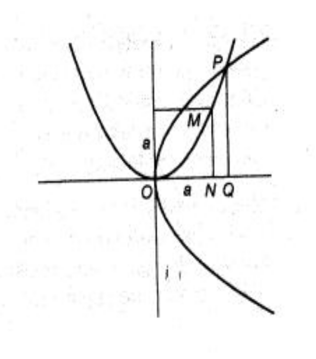
The duplication of the cube: while the problem is without solution using row and compact, i.e. circles and straight segments, it finds solution using other curves, or other tools. Plato, for example, found a solution with the method of graduated rods, flowed and rotated (neusis). Menecmo found another method to duplicate the cube, using two parables (fig 2).

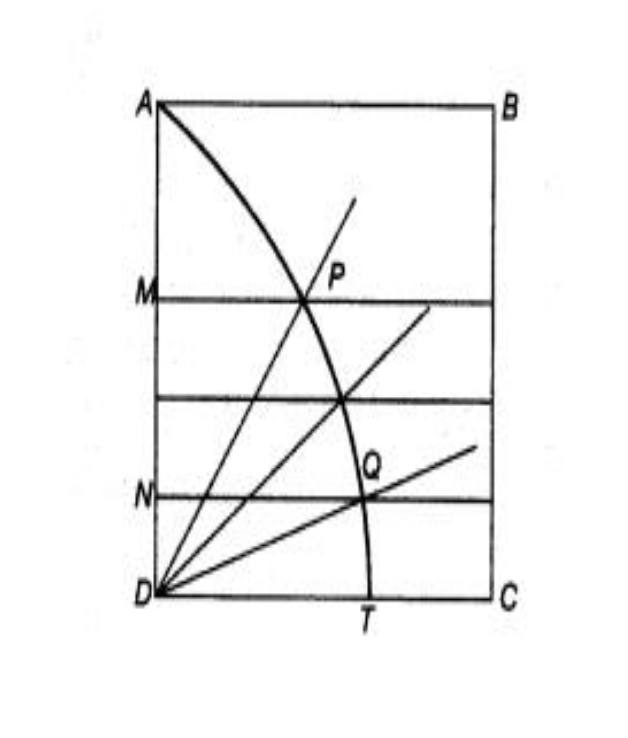
The Ippia trisector (fig 3) serves to divide an angle into three parts; as we mentioned, it is not buildable with line and compact. The curve is achieved by translating the AB segment evenly until it coincides with DC; and at the same time by turning the DA segment evenly until it coincides with DC. The place of the intersection points of the two segments during their movement is the trisector.

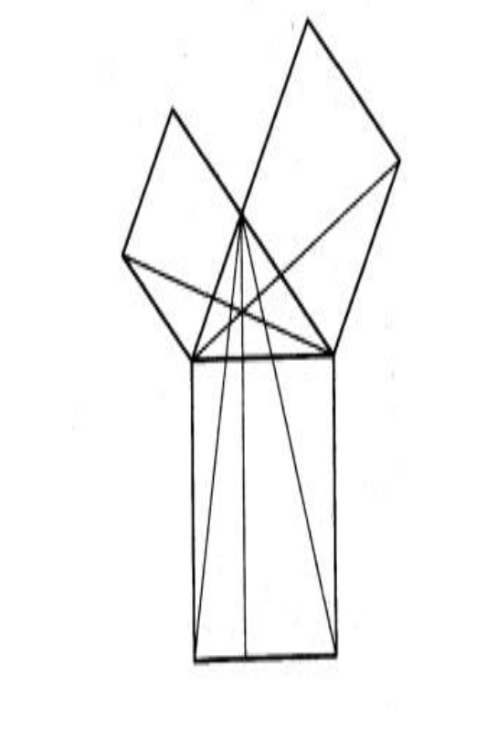
The mill of Euclide (fig 4), taken from proposition 47 of the first book of Elements, also known as chair of the bride or tail of the peacock, lends itself to a simple demonstration of the Pythagorean theorem.

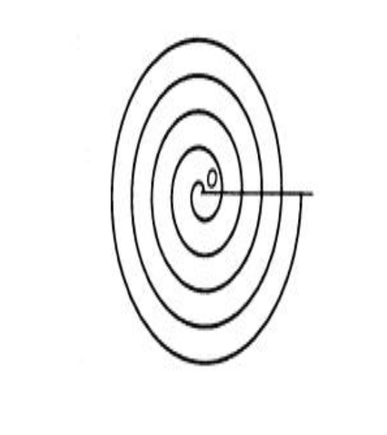
Archimede's spiral (fig 5) is a flat curve, drawn from a point that moves evenly along a semiretta, while this in turn rotates evenly around its extreme. The study of the spiral was probably motivated by the study of the three famous classic problems, and in fact it lends itself easily to the construction of solutions for the trisection of the angle and for the square of the circle.

The circumference is a very rich figure of geometric possibilities, as a creator of countless other curves: stars, hypocycloids and epicycloids and many others. In fact many curves are daughters or close relatives of the circle; starting from it you can unbalance in building many figures, finding in them geometric interest, discovering their hidden properties and calculating their size: it is what the ancient Greeks did when the study of the geometry began. Or you can admire the harmony of proportions, and the grace of graphic representation. Or even, using a computer, you can build figures having as limit only the imagination and ability of the programmer.

Le Conics. If we draw on a glossy circumference and project it from a point on a screen, varying the inclination of it, the circumference can be transformed into a larger or smaller circumference, or into an ellipse, a hyperbole or a parable. Such figures take the name of Conics because they can be obtained by dissecting with a plan a cone with two falde, as is illustrated in Fig.6.

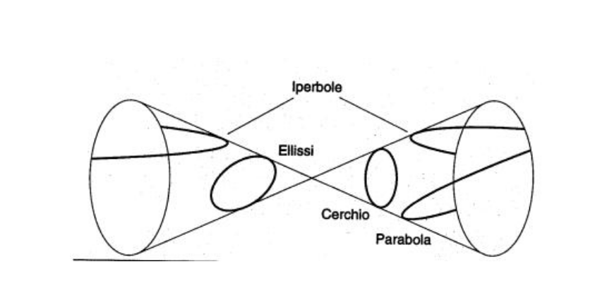
More precisely, the circumferences are obtained if the plane is perpendicular to the cone axis, the ellipses if it is oblique to the axis, the hyperbolites when the plane is parallel to the cone axis and the parables if the plane is parallel to a cone generator. We owe to Apollonius of Perga (III-II century BCE) the broadest study that has come from antiquity, concerning the Conics sections. Apollonius demonstrates among other things a series of properties that will lead to important applications in many fields of science and technology.

The ellipse has in particular two points, which are called fires, located on the greater diameter, such that the sum of distances from the fires is the same for any point on the curve. This fact can be exploited to trace the ellipse, in a rather approximate but sufficient way, for example, to build flower beds in the form of ellipses (not by chance it is called ellipse of the gardener). A second property of the fireworks is that the perpendicular embellished at its own point any divides half the angle formed by the segments that combine this point with the two fires. As a result, a radius of light that starts from one of the fires, and is reflected on the ellipse, passes for the other fire. The same goes for sound waves.

In the circle the fires fall both in the center; as the ellipse stretches, they turn away more and more. The parable no longer has only one fire; the other, so to speak, went to infinity. The rays that come from this fire to infinity are parallel straights; reflecting on the parable they end up in the remaining fire. If we want to concentrate on a parallel beam point, we will have to use a parable-shaped mirror.

What happens with hyperbole is a little more complicated. If we put ourselves outside, a direct radius towards a fire is reflected in the direction of the other fire. Inside, a radius coming from a fire, after a reflection on hyperbole seems to come from the other. The interest in the Conics sections is not limited to these properties, however important. In fact, they enter into the solution of scientific problems that have determined what has been called the “scientific revolution”. In Mathematical Discourses and Demonstrations over two New Sciences, G.Galilei (1564-1642) showed that the trajectory of a bullet is a parable. Another problem, of which the Conics sections have formed the key to achieving a solution, is that of the orbits of the planets.

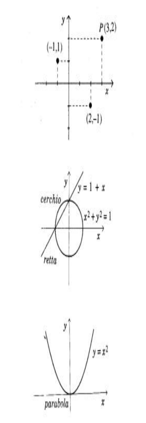
Both the line and the compass, and the Conics sections, are part of the scientific heritage of classical Greece. They are found, it is true, not a few other curves in the works of Greek mathematicians: spirals, quadrants, concoids, cyssoids, but in any case they are particular curves, coming more from the imagination of this or of that geometra than from an internal dynamic of the mathematics. Except for the Conics sections, each Greek curve has characteristics valid for it alone and no other. To get out of this closed world you need a method that applies to all curves without being peculiar to any one. A decisive step is the introduction of the Cartesian coordinates, which take their name from the philosopher and mathematician René Descartes (Cartesio, 1596- 1650). Each P point of the plan can be identified by means of two numbers (x,y), distances from two perpendicular straights. The latter are called Cartesian axes, and the x and y coordinates of the P point. Of the two, x is said the ascissa and y the order; the ascissa takes positive to the right and negative to the left, the positive order up and down (fig 7).

The possibility of studying general methods and procedures makes the new Cartesian setting more agile and more powerful than the construction techniques of classical geometry. Curves can be built by points, solving equations. Conversely, equations can be resolved by means of the intersection of two curves. If the degree of equation is greater than 2, the straights and the circles are no longer enough, and you must resort to curves such as the Conics sections or even other less familiar. As the degree of equation becomes higher, more and more complex curves will be needed.

The possibility to consider “generic” curves poses in a different way many classic problems, in particular that of squares and tangents. If you limit yourself to the line and the compass, very few are the positive results: Hippocrates manages to square the lunules, the first example of exact square of a curvilinear figure; Archimedes discovers the square of the parable. The Greeks had determined the tangent to the circle or the Conics sections, as well as to other particular curves.

In the new Cartesian formulation, the two problems take a different look: no longer to square this or that figure, or to find the tangent to this or that curve, but to identify a uniform method, which allows to trace the tangent to an arbitrary curve, or to give a process to square a figure bound by any curve. The first of these problems, partly solved by Descartes himself, will lead to the discovery of the differential calculation by Newton and Leibniz (1646-1716). The second will be the object of the whole calculation. More difficult is the so-called reverse problem of tangents, or in modern terms the integration of a differential equation.

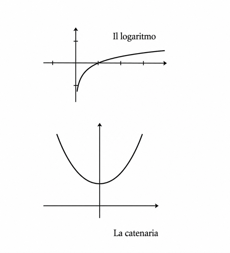
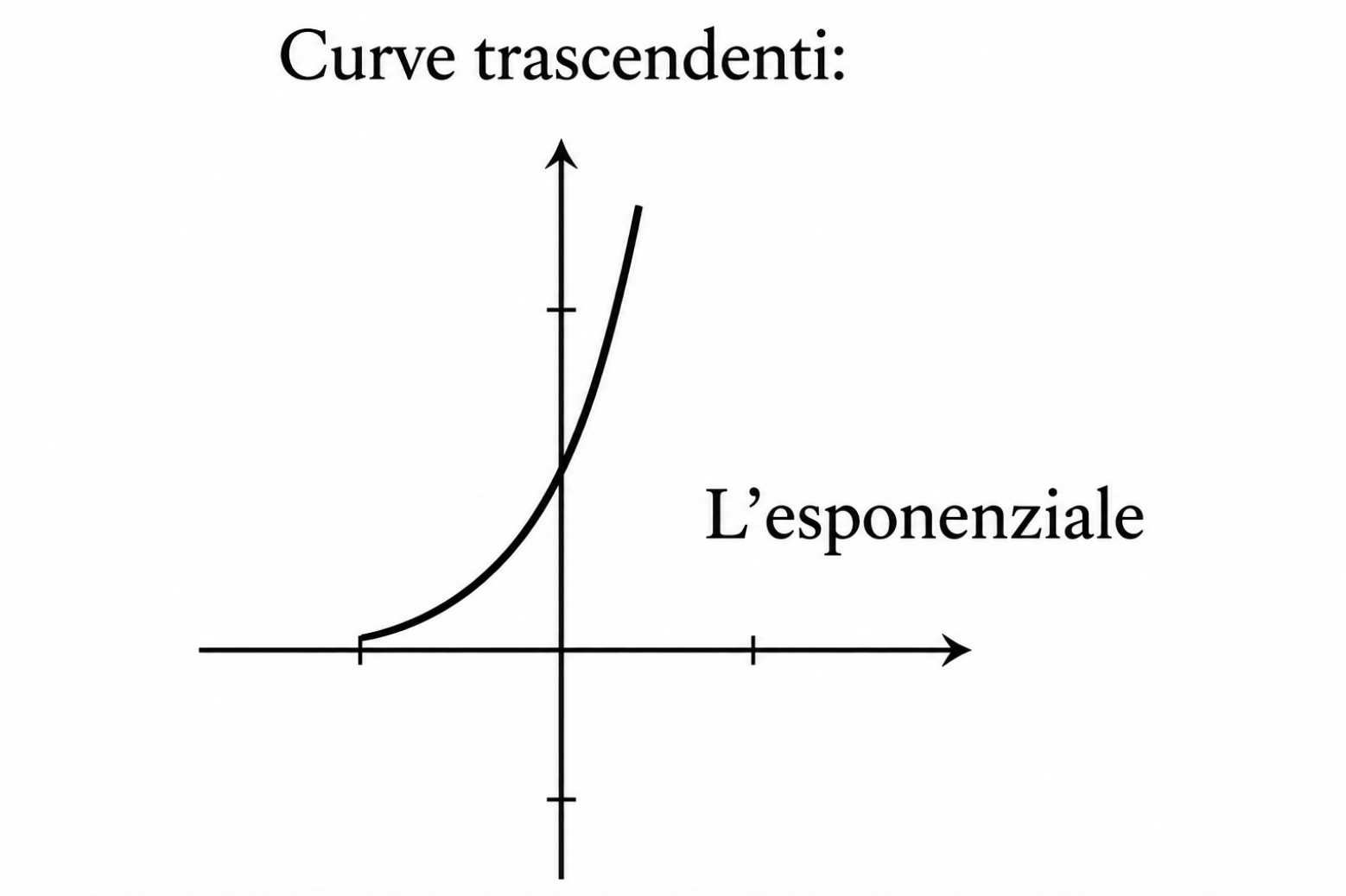
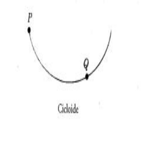
From a geometric point of view, the problem is to find a curve knowing a relationship between its points and relative tangents. Analytically, it results in an equation that binds x and y variables with their differentials. Differential equations lead to a new class of curves, transcendent curves. These curves cannot be expressed through an algebraic equation, but require the introduction of new functions, including trigonometric functions, logarithms, exponentials (fig 8).

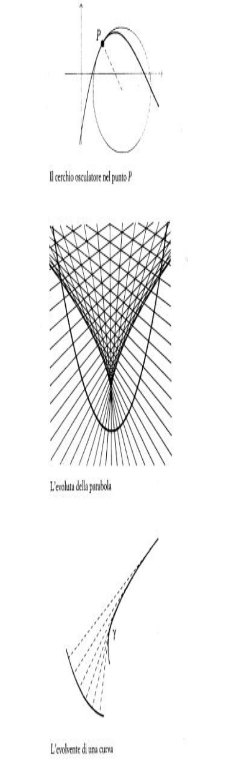
The development of the infinitesimal calculation in the eighteenth century allows to make considerable progress in the study of the properties of the curves. For example: among all the circles passing through P there is one that fits better than others to the curve trend near P. This circle takes the name of the obscure circle. We can thus measure the curvature of a curve. When changing point P on the curve, the warp centers (circles of the obscure centers) will describe a second curve, which is called evolved of the first. This curve is also the envelope of the perpendicular straights at the given curve. Reciprocally, the first curve is the evolution of the second (fig 9).

The evolving-evolving relationship can also be useful to solve technical problems.

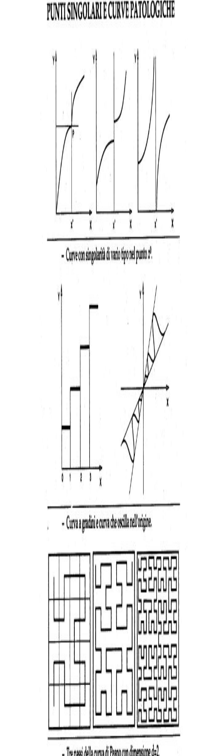
The classic geometry tells us that a body has three dimensions, one surface two and one curve. A curve is called “continue” when it can be drawn with a pen without ever detaching it from the sheet. It may have “singular” points in which there is a discontinuity in the tangent, or a jump that can be finished or infinity (fig 10).

In the first case the curve, in the simple point P(x) admits two tangents, in the second case it has a sharp variation, and finally in the third case we are in the presence of a vertical asymptote. Figure 11 shows the “curva a gradini” and a curve that oscillates more and more when we approach the origin. A real revolution in the geometry was found with the research of G.Cantor (1845-1918) and G.Peano (1858-1932) which built a whole series of geometric monsters (pathological curves) that jeopardized the same foundations of the Euclide geometry, that is the concept of "dimension". In 1890 Peano built his famous curve that fills the square. Figure 12 shows the first three stages of construction of the curve: divide the starting square into an ever larger number of squares, take the center of each of them and connect it with the center of the two adjacent squares. At the limit, the curve will pass for each point of the square and therefore, instead of a size, has two! The debate on the concept of “dimension”, which led to the “fractal spaces” of B. Mandelbrot, having a non-full dimension, was then opened. In this way, we come to the disconcerting conclusion that the “regular curves” (for example circumference and ellipses) are pure geometric abstractions, while the curves considered pathological are those that are actually found in nature. For example, the line of a coastline seems increasingly jagged, as we approach: it is therefore not possible to define the length of the coast in a unique way, it tends to become infinite.

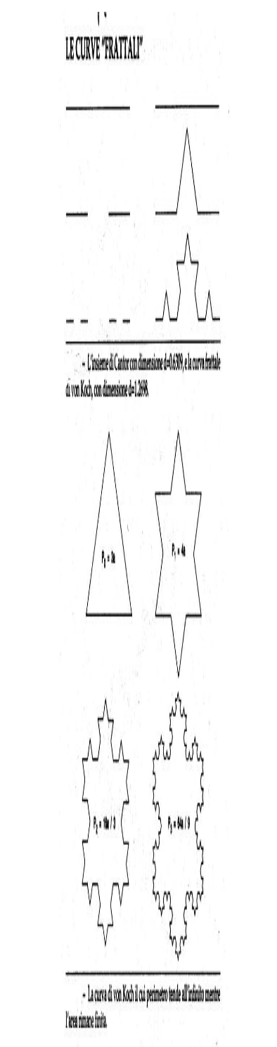
-The Cantor set: given a segment, divide it into three equal parts and then remove the intermediate part (fig 13). Proceeding to infinity with the same method, you get the Cantor set. It is easy to calculate its size: at the first step you have N=3, and you take N=2 segments. After m steps of construction we have: N0 = 3m; N = 2m. You then have the size: d = log 2m/log 3m = log 2/ log 3 = 0,6309. The Cantor set therefore has a smaller size of 1.

-The curve of von Koch: starts from a segment, divides it into three parts, and builds a system of four segments, in the manner indicated in figure 14. It is immediately seen that after m steps of construction there are: N0 = 3m; N = 4m. You then have the size d = log 4m/log 3m = log 4 / log 3 = 1,2698 which is greater than 1.

Particularly interesting is the fractal curve of von Koch, also called snowflake. It is obtained in the manner indicated in Figure 15, and if we indicate with the length of the side of the initial equilateral triangle, the perimeter of the figure, in the successive steps of the construction of the curve, is given by: p0 = 3 a; p’ = 4 a; p’ = (16/3) a and after m steps it is: pm = 3 a (4/3)m

Passing to the limit, when m tends to infinity, the perimeter of the snowflake tends to become infinity, while its area remains over. It is interesting to note that the fractal curve of von Koch does not have tangents, because it changes sharply direction in every point, and therefore it is infinitely irregular.

-The sets of Julia and Mandelbrot (fig 16 and 17). Fractals are a language of balancing, because their fundamental elements cannot be observed directly. They are therefore essentially different from the simple figures of the euclidea plane geometry, such as polygons and circumferences. In fact, fractals are not expressed by primary forms, but by “algoritmi”, i.e. sets of geometric or algebraic procedures, which are then translated into images with computers. The flat algebraic curves can be “linear”, like the straight, which is described by a first-degree equation; then there are the “non-linear” curves described by higher-grade equations (Conics, Cubics...). Similarly, fractals can be linear and non-linear.

In linear fractals the algorithms tell us how to enlarge, shrink or move the initial figure, which always remains autosimilar. Much richer in geometric shapes are non-linear fractals, among which are especially square ones. They were studied since 1918 by the French mathematician G. Julia, and more recently by B. Mandelbrot.

According to Mandelbrot in the study of flat curves there appears a hierarchy of increasing complexity:

• at the first level are the regular curves such as the straight and circumference, which locally confuses with the straight. The classic elementary curves also belong to this level.
• at the second level we can place the classic fractal curves, in which complication does not change when we approach: they can become more or less complicated, but there is an invariance of form compared to distance. We then have a fractal dimension which is between 1 and 2, and this dimension remains the same when we approach the curve.
• at the third level we find the Mandelbrot set: when we approach more and more we recognize in some details what is observed globally. But we have a constant increase in complexity, and we can say that chaos increases, but it has an ordered structure, because it can be mathematically described.

Finally, at the fourth level everything is really chaotic and if we approach it we no longer see in detail what was seen globally, but we observe new and unexpected things. We can conclude that the simplest level was the one studied by the elementary geometry. The second level is of great importance in applications because it is easily found in nature. The third level is the Mandelbrot set, and the fourth corresponds to the most complete and uncontrollable chaos.

With this classification we pass from what is simple and regular to what is extremely chaotic, and then emerge the basic categories of scientific thought, that is the local-global relationship and order-caos. Mandelbrot comes to the unexpected conclusion that these objects that were considered “mostruosis” are indeed what we observe in nature. These forms of order within chaos can be formalized with the methods of geometry fractal.

For a more exhaustive treatment on the fractals we remain at the exhibition I fractali: a self-similar world? Still on display at the Museum of Informatics and History of calculation with the report, except for details, downloadable from the website https://www.museoinformatica.it/.